Concepts
Experiment
An experiment is organized in queries. A query is a statement, that is understood by a Database Management System (DBMS).
Single Query
A benchmark of a query consists of these steps:
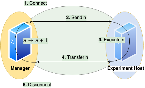
Establish a connection between client and server
This usesjaydebeapi.connect()(and also creates a cursor - time not measured)Send the query from client to server and
Execute the query on server
These two steps useexecute()on a cursor of the JDBC connectionTransfer the result back to client
This usesfetchall()on a cursor of the JDBC connectionClose the connection
This usesclose()on the cursor and the connection
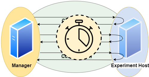
The times needed for steps connection (1.), execution (2. and 3.) and transfer (4.) are measured on the client side. A unit of connect, send, execute and transfer is called a run. Connection time will be zero if an existing connection is reused. A sequence of runs between establishing and discarding a connection is called a session.
Basic Parameters
A basic parameter of a query is the number of runs (units of send, execute, transfer). To configure sessions it is also possible to adjust
the number of runs per connection (session length, to have several sequential connections) and
the number of parallel connections (to simulate several simultanious clients)
a timeout (maximum lifespan of a connection)
a delay for throttling (waiting time before each connection or execution)
for the same query.
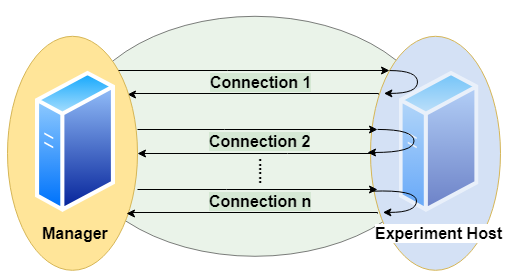
Parallel clients are simulated using the pool.apply_async() method of a Pool object of the module multiprocessing.
Runs and their benchmark times are ordered by numbering.
Moreover we can randomize a query, such that each run will look slightly different. This means we exchange a part of the query for a random value.
Basic Metrics
We have several timers to collect timing information:
timerConnection
This timer gives the time in ms and per run.
It measures the time it takes to establish a JDBC connection.
Note that if a run reuses an established connection, this timer will be 0 for that run.timerExecution
This timer gives the time in ms and per run.
It measures the time between sending a SQL command and receiving a result code via JDBC.timerTransfer
This timer gives the time in ms and per run.
Note that if a run does not transfer any result set (a writing query or if we suspend the result set), this timer will be 0 for that run.timerRun
This timer gives the time in ms and per run.
That is the sum of timerConnection, timerExecution and timerTransfer.
Note that connection time is 0, if we reuse an established session, and transfer time is 0, if we do not transfer any result set.timerSession
This timer gives the time in ms and per session.
It aggregates all runs of a session and sums up their *timerRun*s.
A session starts with establishing a connection and ends when the connection is disconnected.
The benchmark times of a query are stored in csv files (optional pickeled pandas dataframe): For connection, execution and transfer. The columns represent DBMS and each row contains a run.
We also measure and store the total time of the benchmark of the query, since for parallel execution this differs from the sum of times based on timerRun. Total time means measurement starts before first benchmark run and stops after the last benchmark run has been finished. Thus total time also includes some overhead (for spawning a pool of subprocesses, compute size of result sets and joining results of subprocesses). Thus the sum of times is more of an indicator for performance of the server system, the total time is more of an indicator for the performance the client user receives.
We also compute for each query and DBMS
Latency: Measured Time
Throughput:
Number of runs per total time
Number of parallel clients per mean time
In the end we have
Per DBMS: Total time of experiment
Per DBMS and Query:
Time per session
Time per run
Time per run, split up into: connection / execution / data transfer
Latency and Throughputs per run
Latency and Throughputs per session
Additionally error messages and timestamps of begin and end of benchmarking a query are stored.
Comparison
We can specify a dict of DBMS. Each query will be sent to every DBMS in the same number of runs.
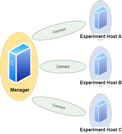
This also respects randomization, i.e. every DBMS receives exactly the same versions of the query in the same order. We assume all DBMS will give us the same result sets. Without randomization, each run should yield the same result set. This tool can check these assumptions automatically by comparison. The resulting data table is handled as a list of lists and treated by this:
# restrict precision
data = [[round(float(item), int(query.restrict_precision)) if tools.convertToFloat(item) == float else item for item in sublist] for sublist in data]
# sort by all columns
data = sorted(data, key=itemgetter(*list(range(0,len(data[0])))))
# size of result
size = int(df.memory_usage(index=True).sum())
# hash of result
columnnames = [[i[0].upper() for i in connection.cursor.description]]
hashed = columnnames + [[hashlib.sha224(pickle.dumps(data)).hexdigest()]]
Result sets of different runs (not randomized) and different DBMS can be compared by their sorted table (small data sets) or their hash value or size (bigger data sets). In order to do so, result sets (or their hash value or size) are stored as lists of lists and additionally can be saved as csv files or pickled pandas dataframes.
Monitoring Hardware Metrics
To make hardware metrics available, we must provide an API URL for a Prometheus Server. The tool collects metrics from the Prometheus server with a step size of 1 second.
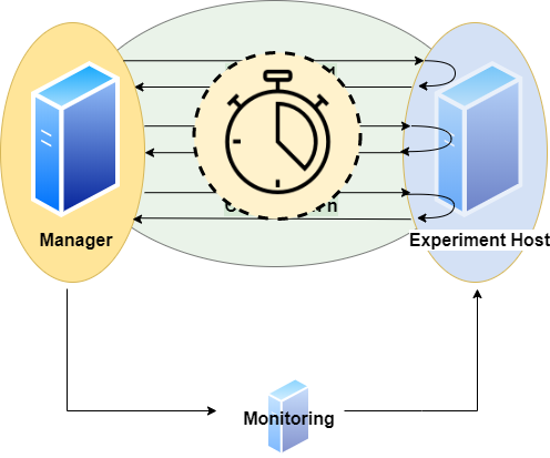
The requested interval matches the interval a specific DBMS is queried. To increase expressiveness, it is possible to extend the scraping interval by n seconds at both ends. In the end we have a list of per second values for each query and DBMS. We may define the metrics in terms of promql. Metrics can be defined per connection.
Example:
'title': 'CPU Memory [MB]'
'query': 'container_memory_working_set_bytes'

'title': 'CPU Memory Cached [MB]'
'query': 'container_memory_usage_bytes'

'title': 'CPU Util [%]'
'query': 'sum(irate(container_cpu_usage_seconds_total[1m]))'

'title': 'CPU Throttle [%]'
'query': 'sum(irate(container_cpu_cfs_throttled_seconds_total[1m]))'

'title': 'CPU Util Others [%]'
'query': 'sum(irate(container_cpu_usage_seconds_total{id!="/"}[1m]))'

'title': 'Net Rx [b]'
'query': 'sum(container_network_receive_bytes_total{)'

'title': 'Net Tx [b]'
'query': 'sum(container_network_transmit_bytes_total{)'

'title': 'FS Read [b]'
'query': 'sum(container_fs_reads_bytes_total)'

'title': 'FS Write [b]'
'query': 'sum(container_fs_writes_bytes_total)'

'title': 'GPU Util [%]'
'query': 'DCGM_FI_DEV_GPU_UTIL{UUID=~"GPU-4d1c2617-649d-40f1-9430-2c9ab3297b79"}'

'title': 'GPU Power Usage [W]'
'query': 'DCGM_FI_DEV_POWER_USAGE{UUID=~"GPU-4d1c2617-"}'

'title': 'GPU Memory [MiB]'
'query': 'DCGM_FI_DEV_FB_USED{UUID=~"GPU-4d1c2617-"}'
Note this expects monitoring to be installed properly and naming to be appropriate. See https://github.com/Beuth-Erdelt/Benchmark-Experiment-Host-Manager for a working example and more details.
Note this has limited validity, since metrics are typically scraped only on a basis of several seconds. It works best with a high repetition of the same query.
Evaluation
As a result we obtain measured times in milliseconds for the query processing parts: connection, execution, data transfer.
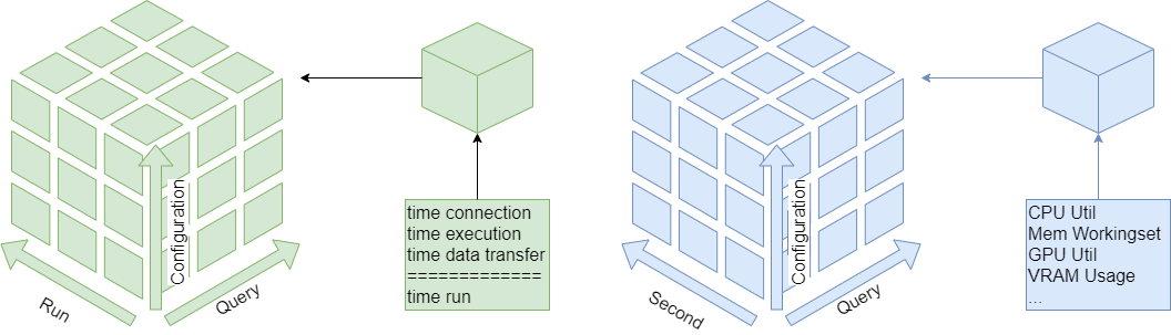
These are described in three dimensions: number of run, number of query and configuration. The configuration dimension can consist of various nominal attributes like DBMS, selected processor, assigned cluster node, number of clients and execution order. We also can have various hardware metrics like CPU and GPU utilization, CPU throttling, memory caching and working set. These are also described in three dimensions: Second of query execution time, number of query and number of configuration.
All these metrics can be sliced or diced, rolled-up or drilled-down into the various dimensions using several aggregation functions for evaluation.
Aggregation Functions
Currently the following statistics may be computed per dimension:
Sensitive to outliers
Arithmetic mean
Standard deviation
Coefficient of variation
Insensitive to outliers
Median - percentile 50 (Q2)
Interquartile range - Q3-Q1
Quartile coefficient of dispersion
First
Last
Minimum
Maximum
Range (Maximum - Minimum)
Sum
Geometric Mean
percentile 25 (Q1)
percentile 75 (Q3)
percentile 90 - leave out highest 10%
percentile 95 - leave out highest 5%
In the complex configuration dimension it can be interesting to aggregate to groups like same DBMS or CPU type.